Exploring AI-Enhanced Development: My Experience with Codeium’s Windsurf IDE

AI-powered tools are transforming the way we code, and I recently got a chance to dive into this revolution with Codeium’s Windsurf IDE. My journey spanned two exciting projects: updating the theme of my mdsinabox.com project and building a Terraform provider for MotherDuck. Each project offered unique insights into the capabilities and limitations of AI-enhanced development. It should be noted that I did pay for the “Pro Plan” as you get rate limited really quickly on the free tier.

Project 1: Updating the Theme on mdsinabox.com

My first project involved updating the theme of my evidence.dev project. Evidence.dev is a Svelte-based app that integrates DuckDB and charting (via ECharts). Styling it involves navigating between CSS, Svelte, TypeScript, and SQL—a perfect storm of complexity that seemed tailor-made for Windsurf’s AI workflows.

I aimed to update the theme fonts to use serif fonts for certain elements and sans-serif fonts for others. Initially, I asked the editor to update these fonts, but it failed to detect that the font settings were managed through Tailwind CSS—a fact I didn’t know either at the time. We wasted considerable time searching for where to set the fonts.

the windsurf editor using cascade (right pane) to update the code

After a frustrating period of trial and error of pouring over project internals, and later reading documentation, I realized that Tailwind CSS controlled the fonts. Once I instructed the editor about Tailwind, it identified the necessary changes immediately, and we were back on track.

updated theme on the nba team pages

However, one gripe remained: Windsurf’s model didn’t include the build files for the Evidence static site, so I had to manually copy files to another directory for it to work. Additionally, debugging errors using the browser’s source view proved more efficient than relying on the editor. These limitations were a bit frustrating, but the experience highlighted the importance of understanding your project’s architecture and guiding AI tools appropriately. Access to a browser emulator would massively improve the debugging experience.

Project 2: Building a Terraform Provider for MotherDuck

The second project was sparked by a potential customer’s request for a Terraform provider for MotherDuck. While I was familiar with Terraform conceptually, I’d never used it before. With the recent launch of our REST API at MotherDuck, this felt like the perfect opportunity to explore its capabilities.

I instructed Windsurf, “I want to make a Terraform provider. Use the API docs at this URL to create it.” The editor sprang into action, setting up the environment and framing the provider. While its initial implementation of the REST API was overly generic and didn’t work, the tool’s ability to see the entire codebase end-to-end made it relatively straightforward to refine. I did have to interject and say “here is an example curl request that I know works, make it work like this” which was enough to get it unstuck.

intervening with cascade to tell it to change directory instead of run go init (again)

As an aside, observing it at times was quite comical as it seemed to take approaches that were obvious incorrect, especially when I was dealing with some invalid authorization tokens. It would almost say “well I trust that my handler has given me a valid token, so it must be something else” and just start doing things that were obviously not going to work.

Anyway, once the main Terraform file was built, I tasked the editor with writing tests to validate its functionality. It recommended Go, a language I had no prior experience with, and even set up the environment for it. Through a mix of trial and error and manual intervention (particularly to address SQL syntax issues like the invalid ‘attach if not exists’ statement in MotherDuck), I managed to get everything working. From start to finish, including testing, the entire process took around four hours—which seemed pretty decent given my experience level.

Conclusion

My experience with Codeium’s Windsurf IDE revealed both the promise and the current limitations of AI-enhanced development. The ability to seamlessly navigate between languages and frameworks, quickly scaffold projects, and even tackle unfamiliar domains like Go was incredibly empowering. However, there were moments of friction—misunderstandings about project architecture, limitations in accessing build files, and occasional struggles with syntax. Getting these models into the right context quickly is pretty difficult with projects that have lots of dependencies and overall my projects are fairly low complexity.

Still, it’s remarkable how far we’ve come. AI-enabled editors like Windsurf are not just tools but collaborative partners, accelerating development and enabling us to take on challenges that might have otherwise seemed impossible. As these technologies continue to mature, I can’t wait to see how I can use them to build even more fun projects.

LLMs in SQL? A real-world application to clean up your CRM data

Executive Summary

Firmographic data, like industry classification, employee count, and location, is notoriously messy and challenging to analyze. Modern databases offer a unique opportunity to clean and maintain this data: by leveraging an LLM, you can synthesize industry information for your accounts directly within a SQL query.

I recently took on exactly this challenge, so this isn’t an abstract solution. I’m using generic data below for data privacy reasons, but this is a real-world solution for a real-world problem I solved for a RevOps team.

h/t to Jacob Matson who demonstrated the underlying concept in MotherDuck:

Problem 1: Maintaining Firmographic Data is a Challenge

One dreaded question for analysts on the sales or revenue team: “quick qq: Can I get our sales broken out by industry?” This question often signals a few late nights spent cleaning up industry data to provide a rough answer to stakeholders who, meanwhile, are wondering, “Why is this taking so long? Don’t we already pay for firmographic data?”

How often does industry data look like this? Way too often.

The never-ending hamster wheel of maintaining firmographic data is a universal challenge. There’s a reason why Dun & Bradstreet took in $2.3B in revenue in 2023 providing this data: it’s not easy to aggregate or keep up to date.

Problem 2: Overwhelming Industry Categories

There is another visible failure point in the chart above: an excessive number of industry categories.

A hidden aspect of any industry cleanup project is narrowing down to a manageable list of 10–15 industry categories. Leave the intricate sub-industries for later—they’re harder to get right, demand 10 times the maintenance effort, and are rarely used. Only address them when there’s a strong business case to do so.

Solving Problem #2, First

Before we can get to the neat LLM-in-SQL work, we need a clear list of industries to ask the LLM to leverage. Usually you want to make this list in collaboration with business, but GPT-4o can generate a solid starting point as well. Here’s the final list I landed on after refining GPT-4o’s starting point to match my preferences::

  1. Technology
  2. Healthcare & Life Sciences
  3. Financial Services
  4. Retail & Consumer Goods
  5. Manufacturing & Industrial
  6. Education
  7. Public Sector & Government
  8. Energy & Utilities
  9. Real Estate & Construction
  10. Transportation & Logistics
  11. Hospitality & Recreation
  12. Professional Services
  13. Nonprofit & Social Impact
  14. Media & Entertainment

Keep in mind, this isn’t a trivial task if your company hasn’t tackled it seriously before. There are a near-infinite amount of industry breakdowns out there, so you need to give purposeful thought to how to group industries based on your own customer base. Your list will likely differ from` others.

Solving Problem #1 Using an LLM in SQL

Now that we have an industry list, it’s time to ask an LLM to help. You could always upload that CSV to ChatGPT and ask it there, but that requires manual steps (download csv / upload to GPT / download csv / upload to DWH) which could get in the way of automating this in the future.

But Snowflake gives us the option to ask an LLM these questions directly in SQL, directly using context from our CRM and other data. Let’s take advantage!

For the test, I found 25 companies in my local area and wrote down only their names. Some are national brands or chains, while others are small mom-and-pop shops and everything in between. This gives me a list like the one below:

OK great! Now we need to get the syntax for querying an LLM in Snowflake. There’s plenty of documentation covering the available LLMs and functions, and the specific function we want to use is Complete. I tested all of the LLMs in Snowflake for this task, and the most consistently accurate one with reasonable processing times was llama3.1-70b, so we’ll use that LLM for now.

Initial LLM code

And here were the results. They are … uh … about what one expects on a first try. Overly verbose.

Pls send help

OK, time to do some “Prompt Engineering” to get this correct, because getting a paragraph for a response is incredibly not helpful.

Specifically, I added a line saying: Only return the industry in each response, I want no other text or explanations.

This works well! Very limited extra text, but it isn’t really categorizing like I want it to. For instance, I consider the After Image Styling Salon to be a Professional Service, not a Retail/Consumer Good.

The LLM would benefit from additional context for each industry for decision making. This is exactly what I would do if giving this task to someone at work. Given ambiguity, both a person and an LLM make arbitrary decisions.

Here’s the adjusted query:

Adjusted query with details for each industry included

The context helped! Notably, I found additional improvement when I described specific decision points in the text. Once I told the prompt that places like Auto Repair and Beauty were Professional Services, it correctly categorized them. Lesson being, if you are sure a specific company type should be in a specific industry, be explicit.

Here’s the new output:

Is this perfect? No. but it’s a great start given that it’s working solely off company name and several of these are small or family-owned.

Green = Match, Red = Not a Match, Yellow = Close

Overall:

  • 16 of the 25 I consider correct or nearly correct (72%)
  • 7 of the 25 I consider incorrect (28%)

Not a bad hit rate for a few minutes of an LLM prompt, with room to improve!

I get why names like “Taco Book” threw the LLM for a loop. That’s a local taco shop, but with the name “Book” in the title and very little online about the company, I get why the coin flip ended up on the side of Retail & Consumer Goods.

What next?

I foresee potential to use additional CRM data to make this approach even more accurate. Company descriptions, headquarters data, sales emails, etc. If it can get to ~7/10 off of name alone imagine the possible improvement with more refined prompt engineering combined with extra data context would .

For example, if you had information in your CRM about Taco Book as a restaurant, the LLM would pick up the industry rather quickly.

This feels like an application of LLMs in SQL that’s only scratching the surface of what is possible. RevOps teams everywhere may soon have a tool to update that pesky CRM data, and surely there are other use cases for this across other domains.

I’d love to hear from you if you are working on something similar!

The ‘e’ in Hex is for ELT

quick note: the justification for doing this is worth like a 17 page manifesto. I’m focusing on the how, and maybe I’ll eventually write the manifesto.

General Approach

This specific problem is loading Point-of-Sale data for a vertical specific system into a database for analysis on a daily basis, but could be generalized to most small/medium data use cases where ~24 hour latency is totally fine.

The ELT pipeline uses Hex Notebooks and dbt jobs, both orchestrated independently with crons. dbt is responsible for creating all tables and handling grants as well as data transformation, while Hex handles extract and load from a set of REST APIs into the database. Hex loads into a “queue” of sorts – simply a table in Snowflake that can take JSON pages and some metadata. Conceptually, it looks like this.

Loading data with Hex

Since Hex is a python notebook running inside of managed infrastructure, we can skip the nonsense of environment management, VMs, orchestration, and so on and just get to loading data. First things first, lets add the snowflake connector to our environment.

Bash
!pip3 install snowflake-connector-python

Now that we have added that package our environment, we can build our python functions. I’ve added some simple documentation below.

Python
import requests
import os
import json
import snowflake.connector
from snowflake.connector.errors import ProgrammingError
from datetime import datetime

# login to snowflake
def snowflake_login():
    connection = snowflake.connector.connect(
        user=SNOWFLAKE_USER,
        password=SNOWFLAKE_PASSWORD,
        account=SNOWFLAKE_ACCOUNT,
        database=os.getenv('SNOWFLAKE_DATABASE'),
        schema=os.getenv('SNOWFLAKE_SCHEMA'),
        warehouse=os.getenv('SNOWFLAKE_WAREHOUSE'),
    )

    # print the database and schema
    print(f"Connected to database '{os.getenv('SNOWFLAKE_DATABASE')}' and schema '{os.getenv('SNOWFLAKE_SCHEMA')}'")

    return connection

# get the last run date for a specific endpoint and store from snowflake
def last_run_date(conn, table_name, store_name):
    cur = conn.cursor()
    try:
        # Endpoints take UTC time zone
        print(f"SELECT MAX(UPDATED_AT) FROM PROD_PREP.{table_name} WHERE store_name = '{store_name}';")
        query = f"SELECT MAX(UPDATED_AT) FROM PROD_PREP.{table_name} WHERE store_name = '{store_name}'"
        cur.execute(query)
        result = cur.fetchone()[0]
        try:
            result_date = datetime.strptime(str(result).strip("(),'"), '%Y-%m-%d %H:%M:%S').date()
        except ValueError:
            # handle the case when result is None or not in the expected format
            try:
                result_date = datetime.strptime(str(result).strip("(),'"), '%Y-%m-%d %H:%M:%S.%f').date()
            except ValueError:
                print(f"error: Cannot handle datetime format. Triggering full refresh.")
                result_date = '1900-01-01'
    except ProgrammingError as e:
        if e.errno == 2003:
            print(f'error: Table {table_name} does not exist in Snowflake. Triggering full refresh.')
            # this will trigger a full refresh if there is an error, so be careful here
            result_date = '1900-01-01'
        else:
            raise e
    cur.close()
    conn.close()
    return result_date

# Request pages, only return total page number
def get_num_pages(api_endpoint,auth_token,as_of_date):
    header = {'Authorization': auth_token}
    total_pages = requests.get(api_endpoint+'?page=1&q[updated_at_gt]='+str(as_of_date),headers=header).json()['total_pages']
    return total_pages

# Returns a specific page given a specific "as of" date and page number
def get_page(api_endpoint,auth_token,as_of_date,page_num):
    header = {'Authorization': auth_token}
    print(f"loading data from endpoint: {api_endpoint}" )
    page = requests.get(api_endpoint+'?page='+str(page_num)+'&q[updated_at_gt]='+str(as_of_date),headers=header).json()
    return page

# Loads data into snowflake
def load_to_snowflake(store_name, source_api, api_key, updated_date, total_pages, conn, stage_table, json_element):
    cur = conn.cursor()
    create_query = f"CREATE TABLE IF NOT EXISTS {stage_table} ( store_name VARCHAR , elt_date TIMESTAMPTZ, data VARIANT)"
    cur.execute(create_query)
    
    # loop through the pages
    for page_number in range(1,total_pages+1,1):
        response_json = get_page(source_api,api_key,updated_date,page_number)
        raw_json = response_json[json_element]
        raw_data = json.dumps(raw_json)
        # some fields need to be escaped for single quotes
        clean_data = raw_data.replace('\\', '\\\\').replace("'", "\\'")
        cur.execute(f"INSERT INTO {stage_table} (store_name, elt_date, data) SELECT '{store_name}', CURRENT_TIMESTAMP , PARSE_JSON('{clean_data}')")
        print(f"loaded {page_number} of {total_pages}")
    
    cur.close()
    conn.close()

# create a wrapper for previous functions so we can invoke a single statement for a given API
def job_wrapper(store_name, api_path, api_key, target_table, target_table_key):
    # get the updated date for a specific table
    updated_date = last_run_date(snowflake_login(), target_table, store_name)
    print(f"The maximum value in the 'updated_at' column of the {target_table} table is: {updated_date}")

    # get the number of pages based on the updated date
    pages = get_num_pages(api_path,api_key,updated_date)
    print(f"There are {pages} pages to load in the sales API")

    # load to snowflake
    load_to_snowflake(store_name, api_path, api_key,updated_date,pages,snowflake_login(),target_table, target_table_key)

Now that we have our python in place, we can invoke a specific API. It should be noted that Hex also has built-in environmental variable management, so we can keep our keys safe while still having a nice development & production flow.

Python
job_wrapper('store_name','api_url',AUBURN_API_KEY,'end_point_name','endpoint_unique_key')

To deploy this for more endpoints, simply update the api_url, end_point_name, and endpoint_unique_id. You can also hold it in a python dict and reference it as a variable, but I found that to be annoying when troubleshooting.

The last step in Hex is to publish the notebook so that you can set a cron job on it – I set mine to run at midnight PST.

Transforming in dbt

I am using on-run-start & on-run-end scripts in my dbt project to frame out the database, in my case, Snowflake.

SQL
on-run-start:
  - CREATE TABLE IF NOT EXISTS STAGING.sales_histories ( store_name VARCHAR , elt_date TIMESTAMPTZ, data VARIANT, id INT) ;

Now that data is in snowflake (in the RAW schema), we can use a macro in dbt to handle our transformation from pages coming from the API to rows in a database. But first we need to define our sources (the tables built in the on-run-start step) in YAML.

YAML
version: 2

sources:
  - name: SOURCE_NAME
    database: DWH_V2
    schema: STAGING
    tables:
      - name: sales_histories

Repeat for each API end point that you want to stage in your database.

Now consider the following model which transforms the JSON pages to rows:

SQL
{{ config(pre_hook="{{ merge_queues( 'sales_histories' , 'STAGING','ticketId' ) }}") }}

select 
    *,
    data:updated_at::datetime as updated_at
from {{ source( 'POSABIT', 'sales_histories' ) }}

Of course, the real magic here is in the “merge_queues” macro, which is below:

SQL
{% macro merge_queues( table_name, schema, unique_id )%}
    MERGE INTO {{schema}}.{{table_name}} t
        USING (
            with cte_top_level as (
            -- we can get some duplicate records when transaction happen as the API runs
            -- as a result, we want to take the latest date in the elt_date column
            -- this used to be a group by, and now is qualify
                select
                    store_name,
                    elt_date,
                    value as val,
                    val:{{unique_id}} as id
                from RAW.{{table_name}},
                lateral flatten( input => data )
                QUALIFY ROW_NUMBER() OVER (PARTITION BY store_name, id ORDER BY elt_date desc) = 1
            )
            select 
                *
            from cte_top_level
        ) s
        ON t.id = s.id AND t.store_name = s.store_name
        -- need to handle updates if they come in
        WHEN MATCHED THEN
            UPDATE SET t.store_name = s.store_name,
                t.elt_date = s.elt_date,
                t.data = s.val,
                t.id = s.id
        WHEN NOT MATCHED THEN
            INSERT ( store_name, elt_date, data, id)
            VALUES ( s.store_name, s.elt_date, s.val, s.id);

    -- truncate the queue
    TRUNCATE RAW.{{table_name}};
{% endmacro %}

A key note here is that snowflake does not handle MERGE like an OLTP database, so we need to de-duplicate it before we INSERT or UPDATE. I learned this the hard way by trying to de-dupe once the data was into my staging table, but annoyingly this is not easy in snowflake! So I had to truncate and try again a few times.

Now that the data is in a nice tabular format, we can run it like a typical dbt project.

Let me know if you have any questions or comments – you can find me on twitter @matsonj

Other notes

There are lots of neat features that I didn’t end up implementing. A noncomprehensive list is below:

  • Source control + CI/CD for the Hex notebooks – the Hex flow is so simple that I didn’t feel this was necessary.
  • Hex components to reduce repetition of code – today, every store gets its own notebook.
  • Using mdsinabox patterns with DuckDB instead of Snowflake – although part of the reason to do this was to defer infrastructure to bundled vendors.

Passing dynamic parameters to SQL Server stored procedures with dbt

If you are using SQL Server with dbt, odds are that you probably have some stored procedures lurking in your database. And of course, the sql job agent is probably running some of those on a cron. I want to show another way to approach these, using dbt run-operations and GitHub actions. This will allow you to have a path towards moving your codebase into a VCS like git.

Unwrapping your wrapper with jinja

The pattern I am most familiar with is using the sql agent to run a “wrapper”, which servers to initialize the set of variables to pass into your stored procedure. The way I have done this with dbt is a bit different, and split into two steps: 1) writing the variables into a dbt model and 2) passing that query into a table that dbt can iterate on.

Since your model to stuff the variables into a table (step 1) is highly contextual, I’m not going to provide an example, but I will show how to pass an arbitrary sql query into a table. Example below:

{% set sql_statement %}
    SELECT * FROM {{ ref( 'my_model' ) }}
{% endset %}

{% do log(sql_statement, info=True) %}

{%- set table = run_query(sql_statement) -%}

For those of you from the SQL Server world – the metaphor here is a temporary table. You can find more about run_query here.

Agate & for loops

What we have created with the run_query macro is an Agate table. This means we can perform any of the Agate operations on this data set, which is pretty neat! In our case, we are going to use a python for loop and pass in the rows of our table.

{% for i in table.rows  -%}
    {% set stored_procs %}
        EXECUTE dbo.your_procedure
            @parameter_1 = {{ i[0] }}
            , @parameter_2 = {{ i[1] }}
    {% endset %}
    {%- do log("running query below...", info=True)  -%}
    {% do log(stored_procs, info=True) %}
    {% do run_query(stored_procs) %}
    {% set stored_procs = true %}
{% endfor %} 

The clever thing to do here with python is that we can pass multiple columns into our stored procedure, which differs from something like dbt_utils.get_column_values that can also be used as part of a for loop, but only for a single column. In this case we can reference which column to return from our table with variable[n], so i[0] returns the value in the first column in the current row, i[1] returns the second column and so on.

Building the entire macro

Now that we have the guts of this worked out, we can pull it together in an entire macro. I’m adding ‘dry_run’ flag so we can see what the generate SQL is for debugging purposes, without having to execute our procedure. As a side note, you could also build this as a macro that you run as pre or post hook, but in that case you would need to include an ‘if execute‘ block to make sure you don’t run the proc when project is compiled and so on.

-- Execute with: dbt run-operation my_macro --args '{"dry_run": True}'
-- to run the job, run w/o the args

{% macro my_macro(dry_run='false') %}
{% set sql_statement %}
    SELECT * FROM {{ ref( 'my_model' ) }}
{% endset %}

{% do log(sql_statement, info=True) %}

{%- set table = run_query(sql_statement) -%}

{% for i in table.rows  -%}
    {% set stored_procs %}
        EXECUTE dbo.your_procedure
            @parameter_1 = {{ i[0] }}
            , @parameter_2 = {{ i[1] }}
    {% endset %}
    {%- do log("running query below...", info=True)  -%}
    {% do log(stored_procs, info=True) %}
    {% if dry_run == 'false' %}
        {% do run_query(stored_procs) %}
    {% endif %}
    {% set stored_procs = true %}
{% endfor %}  
{% do log("my_macro completed.", info=True) %}
{% endmacro %}

Running in a Github action

Now that we have the macro, we can execute in dbt with ‘dbt run-operation my_macro’. Of course, this is great when testing but so no great if you want this in production. There are lots of ways you run this: on-run-start, on-run-end, as a pre or post-hook. I am not going to do that in this example, but instead share how you can run this a stand alone operation in github actions. I’ll start with the sample code.

name: run_my_proc

on:
  workflow_dispatch:
    # Inputs the workflow accepts.
    inputs:
      name:
        # Friendly description to be shown in the UI instead of 'name'
        description: 'What is the reason to trigger this manually?'
        # Default value if no value is explicitly provided
        default: 'manual run for my stored procedure'
        # Input has to be provided for the workflow to run
        required: true

env:
  DBT_PROFILES_DIR: ./
  MSSQL_USER: ${{ secrets.MSSQL_USER }}
  MSSQL_PROD: ${{ secrets.MSSQL_PROD }}
  MSSQL_LOGIN: ${{ secrets.MSSQL_LOGIN }}
   
jobs:
  run_my_proc:
    name: run_my_proc
    runs-on: self-hosted

    steps:
      - name: Check out
        uses: actions/checkout@master
      
      - name: Get dependencies # ok guess I need this anyway
        run: dbt deps --target prod

      - name: Run dbt run-operation
        run: dbt run-operation my_macro

As you can see – we are using ‘workflow_dispatch’ as our hook for the job. You can find out more about this in the github actions documentation. So now what we have in github is the ability to run this macro on demand with a button press. Neat!

Closing thoughts

One of the challenges I have experienced with existing analytics projects on SQL Server and dbt is “what do I do about my stored procedures”. They can be very hard to fit into the dbt model in my experience. So this is my attempt at a happy medium where you can continue to use those battle tested stored procedures while continuing build out and migrate towards dbt. Github actions is a simple, nicely documented way to start moving logic away from the sql job agent, and you can run it “on-prem” if you have that requirement. Of course, you can always find me on twitter @matsonj if you have questions or comments!

Three steps to handling sharded databases with dbt

A common pattern in scaling production app databases is to keep them as small as possible. Since building production apps is not my forte, I’ll lean on the commentary of experts. I like how Silvia Botros, author of High Performance MySQL, frames it below:

https://twitter.com/dbsmasher/status/1520124723870375937
just keep sharding, just keep sharding…

This architecture presents a unique challenge for analytics engineering because you now have many databases with identical schemas, and dbt sources must be enumerated in your YAML files.

I am going to share the three steps that I use to solve this problem. It should be noted that if you are comfortable with jinja, I am sure there are better, more pythonic ways to solves this problem. I have landed on this solution as something that is easy to understand, fast to develop, and fast to run (i.e. performant).

Step 1: leverage YAML anchors and aliases

Anchors and Aliases are YAML constructions that allow you to reduce repeat syntax and extend existing data nodes. You can place Anchors (&) on an entity to mark a multi-line section. You can then use an Alias (*) call that anchor later in the document to reference that section.

https://www.educative.io/blog/advanced-yaml-syntax-cheatsheet

By using anchors and aliases, we can drastically cut down on the amount of duplicate code that we need to write in our YAML file. A simplified version of what I have is below.

  - name: BASE_DATABASE
    database: CUSTOMER_N
    schema: DATA
    tables: &SHARD_DATA
      - name: table_one
        identifier: name_that_makes_sense_to_eng_but_not_data
        description: a concise description
      - name: table_two

  - name: CUSTOMER_DATABASE
    database: CUSTOMER_N+1
    schema: DATA
    tables: *SHARD_DATA

Unfortunately with this solution, every time a new shard is added, we have to add a new line to our YAML file. While I don’t have a solution off hand, I am certain that you could generate this file with Python.

Step 2: Persist a list of your sharded databases

This next steps seems pretty obvious, but you need a list of your shards. There are multiple ways to get this data, but I will share two of them. The first is getting the list directly from your information schema.

(SQL SERVER)
SELECT * FROM sys.databases;

(SNOWFLAKE)
SELECT * FROM information_schema.databases

You can then persist that information in a dbt model that you can query later.

The second way is to create a dbt seed. Since I already have a manual intervention in step 1, I am ok with a little bit of extra work in managing a seed as well. This also gives me the benefit of source control so I can tell when additional shards came online. And of course, this gives a little finer control over what goes into your analytics area since you may have databases that you don’t want to include in the next step. An example seed is below.

Id,SourceName
1,BASE_DATABASE
2,CUSTOMER_DATABASE

Step 3: Use jinja + dbt_utils.get_column_values to procedurally generate your SQL

The of magic enabled by dbt here is that you can put a for loop inside your SQL query. This means that instead of writing out hundreds or thousands of lines of code to load your data into one place, dbt will instead generate it. Make sure that you have dbt_utils in your packages.yml file and that you have run ‘dbt deps’ to install it first.

{% set source_names = dbt_utils.get_column_values(table=ref('seed'), column='SourceName') %}
{% for sn in source_names %}
  SELECT field_list,
    '{{ sn }}' AS source_name
  FROM {{ source( sn , 'table_one' ) }} one
    INNER JOIN {{ ref( 'table_two' ) }} two ON one.id = two.id
  {% if not loop.last %} UNION ALL {% endif %}
{% endfor %}

In the case of our example, since we have two records in our ‘seed’ table, this will create two SQL queries with a UNION between them. Perfect!

Now I have scaled this to 25 databases or so, so managing it by hand works fine for me. Obviously if you have thousands of databases in production in this paradigm, running a giant UNION ALL may not be feasible (also I doubt you are reading this article if you have that many databases in prod). In fact, I ran into some internal constraints with parallelization with UNION with some models, so I use pre and post-hooks to handle it in a more scalable manner for those. Again, context matters here, so depending on the shape of your data, this may not work for you. Annoyingly, this doesn’t populate the dbt docs with anything particularly meaningful so you will need to keep that in mind.

(SQL SERVER)

{{ config(
    materialized = "table",
    pre_hook="
      DROP TABLE IF EXISTS #source;
      CREATE TABLE #source
      (
        some_field INT
      );

      {% set source_names = dbt_utils.get_column_values(table=ref('seed'), column='SourceName') %}
      {% for sn in source_names %}
        SELECT field_list,
          '{{ sn }}' AS source_name
        FROM {{ source( sn , 'table_one' ) }} one
          INNER JOIN {{ ref( 'table_two' ) }} two ON one.id = two.id
       {% endfor %} 
       DROP TABLE IF EXISTS target;
       SELECT * INTO target FROM #source",
    post_hook="
      DROP TABLE #source;
      DROP TABLE target;"
  )
}}    

SELECT * FROM target

So there you have it, a few ways to pull multiple tables into one with dbt. Hope you found this helpful!

Alternative methods: using dbt_utils.union_relations

In theory, using dbt_utils.union_relations can also accomplish the same as step 3, but I have not tested it that way.

Connect Snowflake to Excel in Minutes

Data “Self-Serve” is a buzzword that’s managed to stick around for a long time without a solution. However, I’m convinced that we can get partway there with simple data products rooted in familiar tools. One ubiquitious tool? Excel. Nearly everyone uses spreadsheets or similar productivity tools at work.

That leads me to meet stakeholders where they’re at: in Excel. And modern data warehouses like Snowflake make it really easy to do so. It’s an easy win if you’ve invested in Analytics Engineering to create clean datasets in your database. Let’s bring those datasets to your users.

Here’s how to connect Snowflake into Excel and enable live connections pivot tables in minutes. These are instructions for Windows specifically.

Step by Step Instructions

(1) Install the ODBC Driver

Click on the “Help” button in the Snowflake UI, go to “Download…” and select “ODBC Driver” and “Snowflake Repository”. Install from the file that downloads.

(2) Configure ODBC Driver

Go to your start menu and type in “ODBC” and click on ODBC Data Sources (64 bit)

Under User DSN, select Add…

Select SnowflakeDSIIDriver from the menu

Fill in the boxes as follows – though your individual situation may vary. My example uses SSO when an organization doesn’t allow direct usernames/passwords for Snowflake. Lots of options here and Snowflake has full documentation of options here.

Note: I found that lots of databases & schemas are available even after choosing some here. Not sure the full limitations, so you can play with options. I put all options in for the primary database I cared about and it worked fine.

Click on Test… to confirm it worked. Here’s the dialog if it did:

(3) Connect to database in Excel

Open Excel and go to the Data tab, click on Get Data and choose From Other Sources and pick From ODBC

From the window that pops up, pick the Snowflake connection and select OK

If successful, you’ll see a window with a dropdown showing your available databases. Use that dropdown to pick the database you want.

IMPORTANT: There is an easy way to load data directly into a Pivot Table at this point (thanks Jacob for this tip!) which will save you and teams time.

Once you select the database / schema / table you want, go to that “Load” button on the bottom and click the little down arrow next to it. Choose “Load to…”

The next menu that pops up will give you various options – pick the second one down saying PivotTable Report

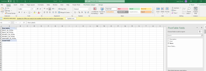
DONE. You’re there. The data is now connected live to Snowflake and is available to pivot. I used Snowflake’s sample “Weather” table which I just learned has basically nothing in it, but that’s besides the point.

Parting notes

There are a couple interesting tidbits to pass both to your stakeholders as well as anyone concerned about Snowflake compute cost & data security.

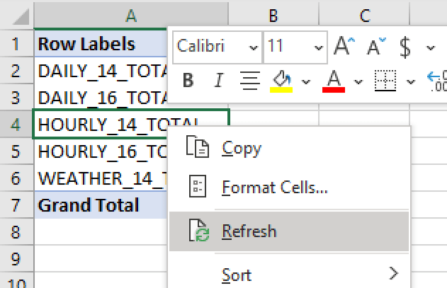
(1) Stakeholders can refresh data live from Snowflake any time. By right-clicking the pivot table and selecting “Refresh”. No more stakeholders asking you for the latest data – they can just get it anytime.

(2) Data is cached on the local machine, reducing compute costs & keeping things snappy for stakeholders. This satisfies worries from both stakeholders on performance (it’s REALLY snappy, even for huge tables) as well as those concerned on cost (compute only happens on refresh).

That’s it! Just a few installations and clicks and you’ve connected Snowflake live into Excel for any stakeholder. Happy self-serving.

Write Code Last – 4 steps to better dashboards

I gave a talk last week about “Data to Dashboard” and I wanted to share it here, too. There is a lot of discussion in the analytics space about dashboards and how to make them look good but less about how to get to that point. This is my take on the subject – I hope you enjoy it.

Toronto Data Workshop – 6/18/2021

Medium Data: MS edition

This video is for your data that is too big for an excel spreadsheet and too small for a data warehouse. I like to refer to this as “Medium Data”.

I can think of many times I needed this during my career. Typically, the “medium data” scenarios were related to snapshotting historical data weekly and showing changes in trends over time. One good trick I learned in one of my first jobs was to snapshot my CRM order book every week and save it in a CSV format. Eventually, that got too large for my meager tools, and I started aggregating, losing data, or other hacks (i.e., multiple excel files). Linking excel files together was basically enough to motivate me to learn SQL. With Azure, you can easily scale into the next size of data and keep your analytics rolling. Check the video below for a 15 min walk through.

Going from CSV to SQL in 16 minutes

I’ve just shown the basics – but there are some awesome articles out there that can go more in-depth, including some great automation.

The core tutorial in this video can be found here: https://social.technet.microsoft.com/wiki/contents/articles/52061.t-sql-bulk-insert-azure-csv-blob-into-azure-sql-database.aspx

To really amp it up with automatic import, check out this: https://marczak.io/posts/azure-loading-csv-to-sql/